19. If I had a nickel for every time I tried creating Pokémon with diffusion 🌀
Github repo for Pokémon sprite generation: Pixelart Diffusion
Prologue
GenAI is one of the hottest topics of the 2020s. Image generation with diffusion models like DALL-E 2 and Stable Diffusion piqued the interest of some, but with the release of ChatGPT, everyone was hooked on generative AI. When speaking of generative AI, most people think of LLMs and text prediction. But the topic of today is actually another family of generative models called latent variable models. These are probabilistic models built around hidden (latent) variables, and they are naturally reasoned about using the Bayesian framework. This family includes many image generation models, such as VAEs and diffusion models.
This post will cover how generative models work, most notably the latent variable models, and then I show an example of a simple diffusion model used for creating custom Pokémon sprites. One of my first projects for this blog was to create an image of “Charizard” using Stable Diffusion with textual inversion, but the image generation model is built from scratch. This post is mostly about theory, with the actual project work being only a minor part of it.
Generation vs. prediction
A large portion of machine learning models are inherently probabilistic in the way that they model the relation between an observed input \(x\) and its target \(y\). Here, we distinguish between discriminative models and generative models. A discriminative model describes the conditional distribution \(p(y\mid x)\), which could be a class \(y\), based on some input \(x\). A generative model tends to describe either the marginal distribution \(p(x)\), the conditional distribution \(p(x\mid y)\), or even the full joint distribution, \(p(x,y)=p(x\mid y)p(y)\). These are all distributions of the data \(x\), some impacted more or less by a target label \(y\). In essence, discriminative models are used for predicting outcomes, and generative models are used for generating data.
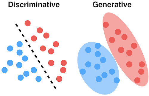
So, in both cases, the internal state of a model describes how the data is structured (or “distributed”), but is done so differently depending on the task. For classification, you would condition on some observed data, and then define the distribution of the outputs, by explicitly defining the probability of each possible output class. For generation, we need a way to describe how the observed data is distributed, while usually taking some target label into account as well, as these are naturally linked.
How do we define a distribution?
In the classification case, all the classes are assigned a probability, given some input. These probabilities sum to 1 and are non-negative, which describes a probability distribution. A linear regression model only outputs a single number ( a point estimate), but can be interpreted as a Gaussian distribution around the estimate, with the residuals determining the variance.
It is not as straightforward with generative models. For classification, you might want to estimate the probability between 10 classes, whereas with generative models you should in theory apply a probability to any possible, let’s say, image (of a fixed resolution). Defining such a distribution is therefore less straightforward, and there are many approaches to this. LLMs model how text works, which results in a probability distribution over the next token, given all the previous ones. Every variable here is observed: the distribution is defined directly over the tokens themselves. Variational Autoencoders (VAE) take a different route. They introduce a hidden latent variable \(z\), a compressed code that the image is generated from. When you sample \(z\), the output is (the mean of) a Gaussian distribution over pixels \(p(x\mid z)\). Diffusion models are also latent variable models, although their latents are less obvious: they are the increasingly noisy versions of the image. By predicting which noise is added to an image, we can move towards a clean image by iteratively predicting slightly cleaner images, where each step in this process is approximately Gaussian.
The point is that a distribution, in a generative model, is rarely explicitly defined as a nice function over the entire space of possible outputs (LLMs are one exception to this, as the probability of a full text is available, by multiplying the probabilities of each token in the chain). In theory, we do want that full distribution, but since the goal is just to generate data, we often use roundabout ways instead. Broadly, generative models either define the distribution directly over the data, like LLMs, or introduce latent variables and define it through them: \(p(x)=\int p(x\mid z)p(z)\,dz\). This second group, latent variable models, is the focus of this post, and the natural tool for reasoning about them is the Bayesian framework, covered next.
The math behind latent variable models: Probability theory and Bayes theorem
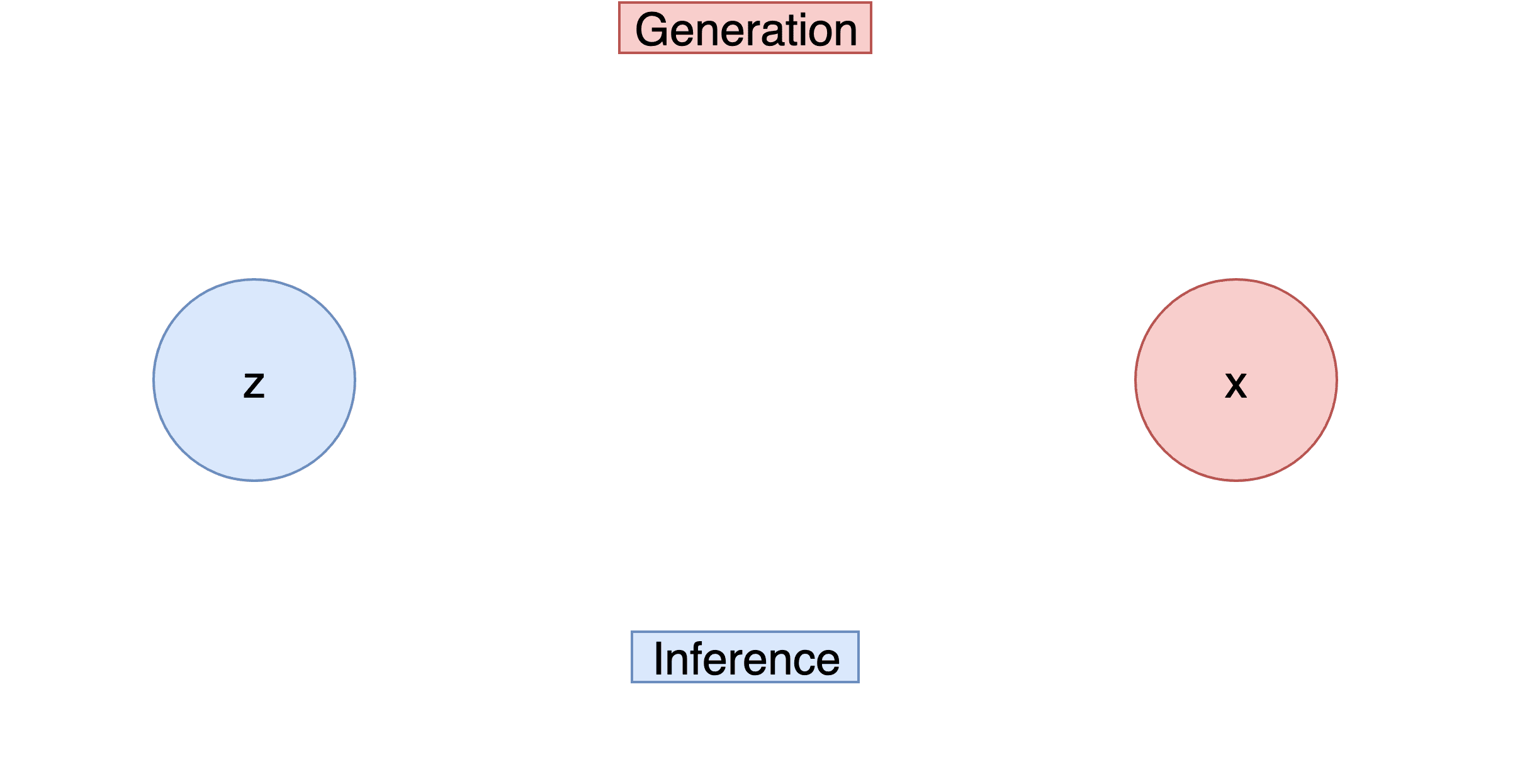
Consider the image prompt: “Dog running on grass”. This single prompt shouldn’t always produce the same output, since there can be many relevant images of dogs running on grass. The prompt defines the concept, but leaves a lot undecided: the breed, the pose, the color of the fur, the lighting, the camera angle. This remaining variation can be captured by a set of latent variables \(z\), and by sampling different latents, many possible images can be generated from the same prompt. Some outputs are obviously more likely than others, but never certain. This is exactly where probability theory comes in, and especially the Bayesian framework. If a generative story explains how some hidden causes \(z\) produce some data \(x\), then the Bayesian framework is meant to reverse that process: given observed data, which hidden causes are most plausible? In our example, the latents might encode how fluffy the dog is, how it is positioned, or how green the grass is (among other things), although in practice the latents are rarely human-interpretable, and are usually much more abstract. The math behind this is neatly captured by Bayes Theorem/Rule, which follows simple rules from probability theory:
\[p(z\mid x)=\frac{p(x,z)}{p(x)}=\frac{p(x\mid z)p(z)}{p(x)}\]Let’s dissect this. \(p(z)\) is our prior assumption about how the latents behave. Since we create the models, we can define the role of the latents. For a VAE, we design the latents to be Gaussian, because this property makes modeling easier. Next, \(p(x\mid z)\) is the likelihood of our data being produced by some latent. Then \(p(x)\) is the marginal distribution (or “evidence”) of the data, meaning the data distribution without conditioning on the latents. This quantity is usually intractable to compute, which becomes apparent later. At last, we have \(p(z\mid x)\), which is the posterior distribution of latents, given the observed data. It answers the question: “which latents could plausibly have produced our data?” Note that this is a distribution, not a single answer, since several latents might explain the same image.
An example
These definitions may feel abstract on their own, so let’s try an example. Consider a VAE trained on just dog images. The prior \(p(z)\) describes the latent space, which we define to be a standard Gaussian \(\mathcal{N}(0,I)\). The likelihood \(p_{\theta}(x\mid z)\) is the decoder, a network with parameters \(\theta\) that takes a latent \(z\) and outputs the mean of a Gaussian over pixels. The evidence \(p_{\theta}(x)\) describes how likely the model thinks a given dog image is, averaged over all latents. It is defined using quantities that we do know, the prior and the likelihood:
\[p_{\theta}(x)=\int p_{\theta}(x,z)\,dz=\int p_{\theta}(x\mid z)\,p(z)\,dz\]But as you may have noticed, computing this integral is intractable. The latent \(z\) is continuous and high-dimensional, and the decoder is a nonlinear network, so the integral has no closed form, and there are far too many possible latents to simply enumerate them.
This motivates approximating the integral instead. The simplest idea is Monte Carlo sampling: draw many latents from the prior and average the likelihood, \(p_{\theta}(x)\approx\frac{1}{N}\sum_{i=1}^{N} p_{\theta}(x\mid z_i)\) with \(z_i\sim p(z)\). In theory this works, but in practice almost none of the sampled latents decode into anything resembling our specific dog image, so nearly every term is close to zero and the estimate is useless. What we really want is to only sample latents that are relevant for \(x\), which is exactly the posterior \(p(z\mid x)\): the very thing we couldn’t compute in the first place. The VAE’s solution is to learn an approximation of it, namely the encoder \(q_{\phi}(z\mid x)\), a network that maps an image to a Gaussian over the latents that plausibly produced it. Using the encoder to guide the sampling, one can derive a lower bound on the (log) evidence, called the evidence lower bound (ELBO):
\[\log p_{\theta}(x)\geq \underbrace{\mathbb{E}_{q_{\phi}(z\mid x)}\left[\log p_{\theta}(x\mid z)\right]-\mathrm{KL}\left(q_{\phi}(z\mid x)\,\|\,p(z)\right)}_{\text{ELBO}}\]The first term rewards the decoder for reconstructing the image from latents proposed by the encoder. The second term keeps those latents close to the prior, so that sampling from \(\mathcal{N}(0,I)\) at generation time produces meaningful images. Maximizing the ELBO trains the encoder and decoder together, without ever computing the intractable integral.
Note that our goal was never the posterior, but the evidence \(p_{\theta}(x)\). The posterior was just a necessary detour: the ELBO is essentially Bayes’ rule rearranged to solve for the evidence, with the intractable posterior replaced by the encoder:
\[\log p_{\theta}(x)=\text{ELBO}+\mathrm{KL}\left(q_{\phi}(z\mid x)\,\|\,p_{\theta}(z\mid x)\right)\]The KL term is never negative, so the ELBO always sits below the true log evidence, and the gap is exactly how far the encoder is from the true posterior. Maximizing the ELBO therefore makes the data more likely and the encoder more accurate at the same time. And once training is done, neither is needed for generation: we simply sample \(z\sim\mathcal{N}(0,I)\) and decode.
What about diffusion?
Diffusion models fit into the same picture. Their latents are the increasingly noisy versions of the image, \(x_1,\dots,x_T\), where \(x_T\) is pure Gaussian noise and plays the role of the prior. Generation runs this chain backward, with a network removing a little noise at each step, \(p_{\theta}(x_{t-1}\mid x_t)\). The big difference from the VAE is the encoder: instead of learning \(q_{\phi}\), diffusion uses a fixed process that gradually adds Gaussian noise to a real image, so there is no approximate posterior to train. The training objective is still an ELBO, which conveniently simplifies to a very simple task: predict the noise that was added to an image.
This concludes our walkthrough of latent variable models. Now, let’s move to something that is probably more tractable: generating Pokémon sprites.
Pokémon
Just to have something cool to look at, I trained a diffusion model to create sprites of Pokémon. This was initially supposed to be used for an app idea closely related to Pokémon GO with custom sprites, but I put that project on the shelf. Instead, I got to dive more into diffusion models, which then got me to geek out on generative models - something which fascinated me during my last few semesters of university. But anyway.
I know that image models require a bunch of training data, but the current Pokédex only has around 1,000 unique Pokémon (with up to a few sprites per Pokémon). Instead I went to a community that creates fusions of these sprites, which has resulted in a dataset of 260,000 unique sprites in the same art style, each with associated types for conditioning as well.
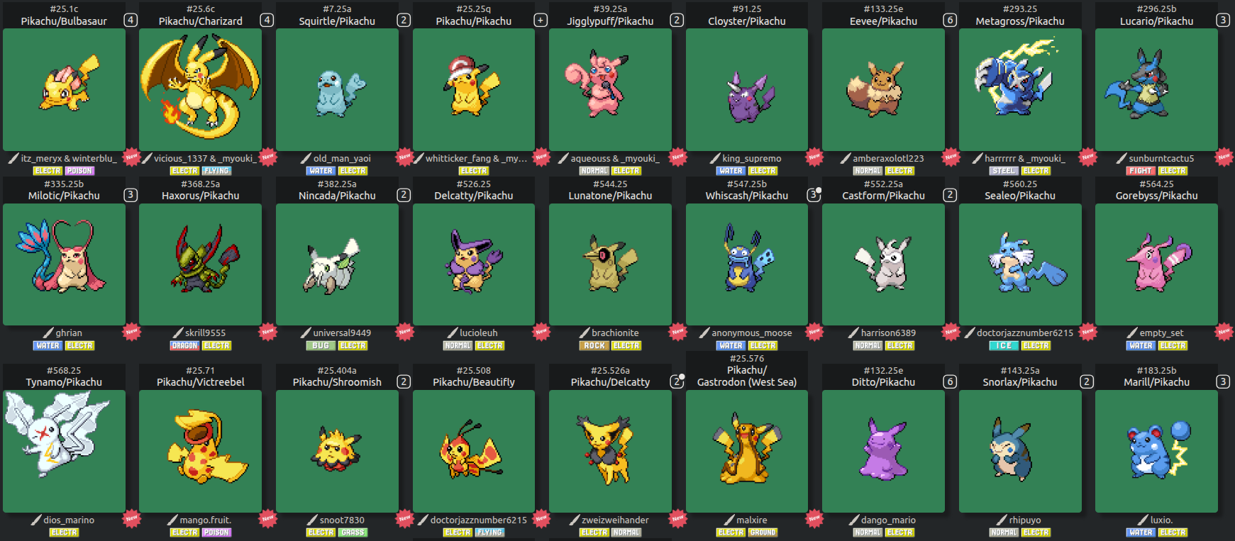
The model used was a simple Denoising Diffusion Probabilistic Model (DDPM) with T=1000, meaning 1,000 latent steps between pure noise and a finished sprite, along with a cosine scheduler, a DPM++ SDE sampler with 50 steps, and classifier-free guidance. There were many variants to go for, such as DDIM models or Latent Diffusion. The goal was just to stitch something together in order to generate an unlimited number of Pokémon. But as it turns out, I did not get that:
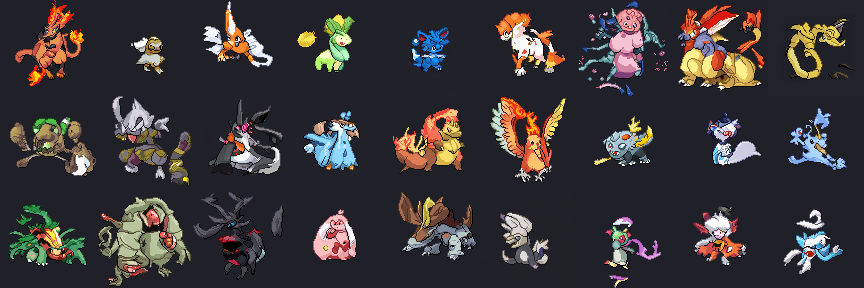
I do like these sprites, as they keep the art style, and even seem to have a transparent background (because I included the alpha channel in training as well). They do look like Pokémon from a distance, but getting closer to them, they remind me of that one image of oddly familiar objects, where you can’t name a single one of them:
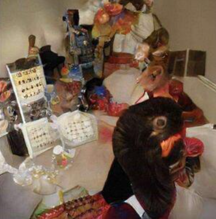
They just don’t quite have it. The art style is there, which is modeled very well. But since Pokémon look so different, and are not natural phenomena, it might be hard to model the full distribution. One option could be to not just condition on types, but also on the base Pokémon themselves, such as labeling all fusions involving a “Pikachu” as having the “Pikachu” label. Anyway, I just wanted to share this. See ya!