3. RAG model for Danish court trial data (Part 1/2)

June 2025 ☀️

Prologue

Ethics regarding the use of AI for decision making in court, has been one of my favorite topics to discuss, as the philosophy of intelligence, conciousness, and emotions in AI has had a big impact on my world view.

As an engineer, I would also like to see things in practice, rather than just theorize about things. This is what drove me to start a project about AI with public Danish court trial data. Ideally, the available data would be structuered in a way similar to datasets in supervised learning, where we have a text description of the case, and a label corresponding to the punishment. Unfortunately, this was not the case, as the data consists of text documents that are not defined in a specific template. Therefore, the goal became to make a RAG model for retrieving these court documents based on a search prompt. I.e. to do natural text search on these documents. I want to do this using local models, and without LLM-pipeline libraries like LangChain.

As the ambition level of the project fell, I had to challenge myself in another way to keep it exciting. I chose to utilize cloud computing for every step of the project, including testing, data processing, storage, and even endpoint hosting, primarily using Azure Machine Learning. I have always struggled with using cloud computing succesfully, so this is a perfect chance to give it another shot.

Data Gathering

In Denmark, we recently acquired a public database of court case documents, which are accesible through the website or the API. Although not exhaustive, it contains many cases from recent years. We will use the API to collect a local copy of all the data.

We first need to authenticate:

import requests
from dotenv import dotenv_values
config = dotenv_values(".env")

# Authenticate with the API
url = "https://domsdatabasen.dk/webapi/kapi/v1/autoriser"
headers = {"Content-Type": "application/json"}
body = {"Email": config["username"], "Password": config["password"]}
response = requests.post(url, json=body, headers=headers)

# Check if the response is successful
if response.status_code == 200:
    data = response.json()
    print("Authorization successful!")
    print("User ID:        ", data["userId"])
    print("User Name:      ", data["username"])
    print("Issued UTC time:", data["issuedUtcTime"])
    token = data["tokenString"]
    print("Token:          ", token)
else:
    print("Error:", response.status_code, response.text)

And then we can fetch the data with a series of GET requests:

headers = {'Authorization': f'Bearer {token}'}
sideNr = 1

while True:
  
    params = {
        'sideNr': sideNr,
        'perSide': 25
    }
    response = requests.get(url, headers=headers, params=params)

    if response.status_code == 200:
        data = response.json()
    ...
    sideNr += 1

# For each page, extract case data
for item in data:

    # For each case, extract documents
    for doc in item['documents']:
        ...

# Extract the HTML content of the document
document = doc['contentHtml']
if not document: continue
all_documents.append(document)

# Use BS4 to extract paragraphs
bs = BeautifulSoup(document, 'html.parser')
text = ''
for page in bs.find_all('div', class_='page'):
    text += page.get_text(separator="\n").strip() + '\n'

# Write each document to a .txt file (both text and HTML)
text_to_txt(text,     f'{texts_dir}/{doc["id"]}')
text_to_txt(document, f'{texts_dir+'_html'}/{doc["id"]}')

# Save meta data
all_meta.append([item['headline'],
                '?'.join([subject['displayText'] for subject in item['caseSubjects']]),
                int(item['id']),
                int(doc['id']),
                doc['displayTitle'],
                doc['verdictDateTime'],
                item['closedCourtroom'],
                item['profession']['displayText'],
                item['instance']['displayText'],
                item['caseType']['displayText']
                ])

The filters available in the request header is quite limited. We can extract 25 documents per page, which is reasonable, but we are not able to filter by time, or any other relevant attributes. Also, sorting is not possible. This is also why we need to extract every document, since we can’t guarantee which document we get otherwise.

I have added a small overview of all the important attributes. Some of them are attributes for the case, while some are attributes of the actual documents associated with a case:

Attribute	Type	Description
headline	case	Headline of the case
caseSubjects	case	Themes/topics of a case (violence, drugs, taxes etc.)
id	case	Unique ID for a case
id	document	Unique ID for a document
displayTitle	document	Title of document
verdictDateTime	document	Time of verdict (as defined in the document)
closedCourtroom	case	Whether the courtroom has been closed from public or not
profession	case	Type of case (criminal case, foreclosure etc.)
instance	case	Stage of court (District court, High court, or Supreme) court
caseType	case	More specifically what category the case is

Data Processing

So, we split the response data into the meta data and the document data. The meta data can easily be described in a table, and will therefore be saved as a parquet-file (instead of csv) in order to save disk space. To further optimize space/memory usage, the column data types are selected manually.

# Convert data types for efficiency
df_meta['id']           = df_meta['id'].astype('uint32')
df_meta['doc_id']       = df_meta['doc_id'].astype('uint32')
df_meta['verdict_date'] = pd.to_datetime(df_meta['verdict_date'])
df_meta['doc_type']     = df_meta['doc_type'].astype('category')
df_meta['profession']   = df_meta['profession'].astype('category')
df_meta['instance']     = df_meta['instance'].astype('category')
df_meta['case_type']    = df_meta['case_type'].astype('category')

# Save to .parquet
df_meta.to_parquet('meta.parquet', index=False)

This is a somewhat neglible addition, as the table is ~5000x10. But it’s still a good principle, and I also just learned these tricks from my “Python and High-peformance Computing” course, so I wanted to see it in practice.

As for the actual documents, they are stored in HTML format. The text itself can easily be extracted using the Beautiful Soup (bs4) library. It is also beneficial to split the text into small paragraphs, such that they can later be used for “chunking” (more on that later). It is easy to make these splits, as each actual paragraph is given by the HTML paragraph- or ‘p’ tag.

Now, the most computationally demanding processing step is to convert each of these paragraphs into an embedding vector, which can take multiple hours. We explain the embedding vectors next.

Sentence Embeddings

Building a RAG model requires that we can convert our prompt, as well as the reference material, into a vector representation, such that they can be compared. This representation is formally called an embedding. We need ML embedding models to perform this transformation.

As we are working with a Danish dataset, it is not possible to simply use the default models, as they are usually in English. Even so-called “multi-lingual” models can still struggle with Danish, as the Danish language is quite underrepresented on the internet. My best attempt was to use a model from Huggingface that was explicitly fine-tuned for the Danish language (link). It’s definitely not perfect, but it’s alright.

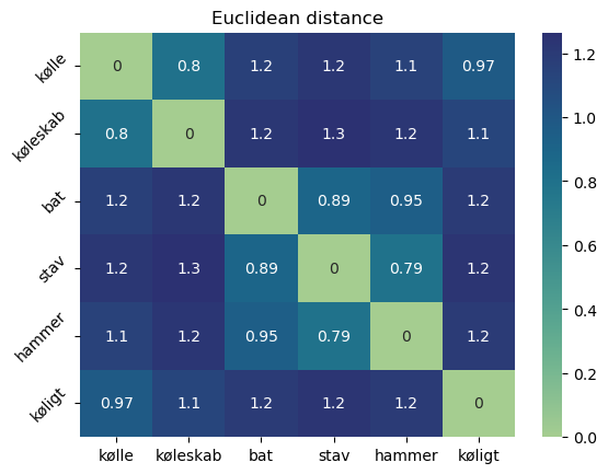
A limitation I have encountered is that the tokenization of words seems a bit wrong. In terms of vector similarity, the word “Kølle” (“club”, as in the weapon) and “Køleskab” (“refrigerator”) are way too similar due to the køl -token. Let’s consider this table of distances between embeddings (meaning that lower values indicate more similarity)

Vector similarity is somewhat complicated, since embeddings might actually be similar in one way, but not the way I want. In the matrix above we see that “bat” (bat), “stav” (rod/stick), and “hammer” (hammer) are somewhat similar to each other, but not similar to “Kølle”.

(Theory) Training an embedding model

Let’s get into a bit more details regarding this embedding model. For basically any NLP (Natural Language Processing) -related task, we should use a transformer-based model. The most popular one would be the GPT-models that are used for the famous chatbots. But GPT-models are inherently text prediction models which are good for generating text, but not necessarily classifying text. On the other hand, BERT-models are good at classification as it takes an entire sequence and analyses each part of the sequence from both left-to-right, but also right-to-left, making them bi-directional (the B in BERT). Our embedding model is therefore a fine-tuned BERT model for (Danish) sentence embeddings, aka. Sentence-BERT.

To optimzie the weights of a deep neural network, we need a loss-function that defines how well the task is being solved during training, in order to nudge the weights in the right direction. This model has been trained using a contrastive loss function, which we need to minimize (but the fraction should be maximzied, so to speak):

Let’s understand this. The training dataset consist of N pairs of sentences, where each element (A and B) in a pair is somehow related to each other. Given the current state of the model, we try to embed A, B, and many other sentences. The goal is the make the embedding of A and B more similar (numerator), while letting A and the other sentences become more dissimilar (denominator). Note that the vector operation between embeddings is the inner product, which is also called the cosine similarity:

This loss is then propagated backwards through the network, and the weights are updated accordingly. Whether sentences are similar or not in the final model is hugely dependent on what the dataset has defined as being similar.

The model we are using is quite light-weight, which was probably to make fine-tuning to the Danish dataset easier. This means that our model embedding-dimension is (only) of size 384, but the maximum sequence (input) length is 512 tokens, which is actually a good amount (~400 words). This should make sure that all of our paragraphs fit individually, but not entire court trial documents.

Recall that our task is to find the trial document that best matches our prompt. We are quite limited by this token size, as we can’t simply embed an entire document into a single vector (that would likely also require a larger embedding size). Instead, we will try and embed each paragraph of the documents, and track which paragraph belongs to which document. This is called “chunking”, for which there are multiple strategies for how to embed these subtexts. We are lucky to already have beautifully split paragraphs in the trial documents, but for long texts, another strategy could be to embed overlapping subtexts of a fixed window-size, and a fixed overlap-size.

RAG Model

Let’s make it completely clear what we want to achieve using this model:

A list of the k most relevant documents wrt. a prompt, given the similarity between the prompt and a single paragraph in these documents.

It is, however, quite common to extend a chat-bot with RAG capabilities, but not necessary. To do this, the RAG model should return some text, which can then be injected into the “system prompt” (not the “user prompt”). A simplified example could be:

USER PROMPT       : "What is the worst punishment a burglar has received?"
<RAG>             : *search for relevant documents*
<RAG>             : *returns [doc_A, doc_B, doc_C]*
SYSTEM            : "Your job is to answer questions about the following court trials: {content of doc_A, doc_B, doc_C}
ASSITANT RESPONSE : "Here is the worst punishment a burglar has received: <...>"

If we were to do this ourselves, we should be cautious of:

1. The quality of the LLM used, due to challenges with the Danish language
2. Which information the RAG returns, as the entire reference document is too large to fit within the system prompt

Anyway, we are keeping it simple.

We have not talked about the challenge of searching for similar documents, which is very interesting. The straight forward way to find the most similar vectors wrt. the prompt vector, would be to simply check all options by brute force. In itself, this is slow, but using the FAISS (Facebook AI Similarity Search) library, many optimizations have been applied to speedup even the brute-force approach. It’s very memory efficient, and it utilizes multiprocessing in order to parallelize the computation. They also offer approximate solutions for large datasets, where brute force in not feasible.

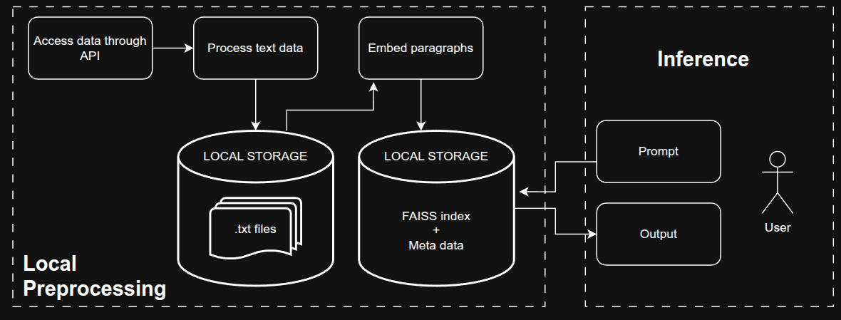
As we have covered all steps of the process, let’s show a over-simplified flowchart: